Carbon Sink at South Pole Has Grown Recently, Historical Collections Reveal
ScienceDaily (Feb. 21, 2011) — By studying collections of a marine bryozoanthat date back to a famous 1901 expedition to the South Pole, researchers have found that those organisms were growing steadily up until 1990, when their growth more than doubled.
The data, reported in the February 22 issue of Current Biology, provide the highest-latitude record of a century of growth and some of the first evidence that polar carbon sinks may be increasing.
The bryozoan in question, known as Cellarinella nutti, is a filter-feeding invertebrate that looks like branching twigs. C. nutti is found in abundance in the Antarctic and is ideal for such studies because it preserves a clear macroscopic environmental record in its skeleton, recorded as tree-ring-like growth-check lines.
"This is one of the few pieces of evidence that life in Antarctica has recently changed drastically," said David Barnes of the British Antarctic Survey. "These animals are taking more carbon dioxide out of circulation and locking it away on the seabed."
The more rapid growth of C. nutti reflects a coincident increase in the regional production of the phytoplankton that the bryozoan eats. Those algae rely on carbon dioxide dissolved into the seawater for their sustenance. The carbon in the algae is taken up by C. nutti, where it is incorporated into their skeleton and other tissues. As the animals grow, portions of it break off and are buried in the seabed. "Thus, the amount of carbon being buried on the seabed is increasing -- whilst globally we are becoming more aware of the need to reduce carbon dioxide in the atmosphere," Barnes said.
He says the shift is most likely the result of ozone losses, which have led to an increase in wind speeds over the last decade. Those stronger winds are a boon to plankton, as they blow ice out of the way and drive greater circulation of surface waters.
"If we are right, this is a rare example of animals responding to one global phenomenon, the ozone hole, and affecting another, the greenhouse effect," Barnes said.
The discovery would not have been possible without early marine collections assembled by the explorer Captain Robert Falcon Scott, a polar pioneer who led the British National Antarctic Expedition and British Antarctic Expeditions at the turn of the 20th century, along with specimens maintained by museums in the United Kingdom, United States, and New Zealand.
"Scott's most famous journey was to reach the South Pole, but a team lead by the Norwegian explorer [Roald] Amundsen beat them to it," Barnes said. "Scott's team died in 1912 on the journey back to his food depots, and so his exploits are often not associated with success. What is not so well known is that his voyages were first and foremost scientific ones, and the collections of material and information they made were impressive even by today's standards."
The findings highlight the challenges of understanding the effects of large-scale processes such as the ozone hole or climate change. "This is not just because it is patchy in space and time, but also because of interactions between effects, as we found," Barnes said.
It is not yet clear how big an impact the changes in C. nutti might have, and at the moment, Barnes suspects it is likely to be quite small.
"Nevertheless, we think that the combination of ice shelf losses and sea ice losses due to climate change and the effect of ozone loss-induced wind speeds offer some hope for much-needed carbon sequestration to the seabed in the Southern Ocean," Barnes said. "There are few other places in the world where global and regional changes could actually lead to more carbon being removed from the system."
Climate Projections Show Human Health Impacts Possible Within 30 Years
New studies demonstrate potential increases in waterborne toxins and microbes harmful to human health
American Association for the Advancement of Science (AAAS) Annual Meeting: Feb. 19 Symposium 10:00 a.m. – 11:30 a.m. (EST)
A panel of scientists speaking today at the annual meeting of the American Association for the Advancement of Science (AAAS) unveiled new research and models demonstrating how climate change could increase exposure and risk of human illness originating from ocean, coastal and Great Lakes ecosystems, with some studies projecting impacts to be felt within 30 years.
“With 2010 the wettest year on record and third warmest for sea surface temperatures, NOAA and our partners are working to uncover how a changing climate can affect our health and our prosperity,” said Jane Lubchenco, Ph.D., under secretary of commerce for oceans and atmosphere and NOAA administrator. “These studies and others like it will better equip officials with the necessary information and tools they need to prepare for and prevent risks associated with changing oceans and coasts.”
In several studies funded by NOAA’s Oceans and Human Health Initiative, findings shed light on how complex interactions and climate change alterations in sea, land and sky make ocean and freshwater environments more susceptible to toxic algal blooms and proliferation of harmful microbes and bacteria.
Climate Change Could Prolong Toxic Algal Outbreaks by 2040 or Sooner
Herrold family harvesting oysters in Willapa Bay, Washington. (Credit: With permission from Bill Dewey, Taylor Shellfish Farms, Inc.)
Using cutting-edge technologies to model future ocean and weather patterns, Stephanie Moore, Ph.D., with NOAA’s West Coast Center for Oceans and Human Health and her partners at the University of Washington, are predicting longer seasons of harmful algal bloom outbreaks in Washington State’s Puget Sound.
The team looked at blooms of Alexandrium catenella, more commonly known as “red tide,” which produces saxitoxin, a poison that can accumulate in shellfish. If consumed by humans, it can cause gastrointestinal and neurological symptoms including vomiting and muscle paralysis or even death in extreme cases.
Longer harmful algal bloom seasons could translate to more days the shellfish fishery is closed, threatening the vitality of the $108 million shellfish industry in Washington state.
“Changes in the harmful algal bloom season appear to be imminent and we expect a significant increase in Puget Sound and similar at-risk environments within 30 years, possibly by the next decade,” said Moore.
“Our projections indicate that by the end of the 21st century, blooms may begin up to two months earlier in the year and persist for one month later compared to the present-day time period of July to October.”
Natural climate variability also plays a role in the length of the bloom season from one year to the next. Thus, in any single year, the change in bloom season could be more or less severe than implied by the long-term warming trend from climate change.
Moore and the research team indicate that the extended lead time offered by these projections will allow managers to put mitigation measures in place and sharpen their targets for monitoring to more quickly and effectively open and close shellfish beds instead of issuing a blanket closure for a larger swath of coast or be caught off guard by an unexpected bloom. The same model can be applied to other coastal areas around the world increasingly affected by harmful algal blooms and improve protection of human health against toxic outbreaks.
More Atmospheric Dust From Global Desertification Could Lead to Increases of Harmful Bacteria in Oceans, Seafood
Aerosolized dust is clearly visible in the satellite image and stretches across the Atlantic Ocean nearly continuously from Western Africa into the Caribbean and Gulf of Mexico.(Credit: With permission from SeaWIFS Project, NASA/Goddard Space Flight Center and ORBIMAGE.)
Researchers at the University of Georgia, a NOAA Oceans and Human Health Initiative Consortium for Graduate Training site, looked at how global desertification — and the resulting increase in atmospheric dust based on some climate change scenarios — could fuel the presence of harmful bacteria in the ocean and seafood.
Desert dust deposition from the atmosphere is considered one of the main contributors of iron in the ocean, has increased over the last 30 years and is expected to rise based on precipitation trends in western Africa. Iron is limited in ocean environments and is essential to most forms of life. In a study conducted in collaboration with the U.S. Geological Survey, Erin Lipp, Ph.D. and graduate student Jason Westrich demonstrated that the sole addition of desert dust and its associated iron into seawater significantly stimulates growth and persistence of Vibrios, a group of ocean bacteria that occur worldwide and can cause gastroenteritis and infectious diseases in humans.
“Within 24 hours of mixing weathered desert dust from Morocco with seawater samples, we saw a 10-1000-fold growth in Vibrios, including one strain that could cause eye, ear, and open wound infections, and another strain that could cause cholera ,” said Lipp. “Our next round of experiments will examine the response of the strains associated with seafood-related infections.”
Since 1996 Vibrio cases have jumped 85 percent in the United States based on reports that primarily track seafood-illnesses. It is possible this additional input of iron, along with rising sea surface temperatures, will affect these bacterial populations and may help to explain both current and future increases in human illnesses from exposure to contaminated seafood and seawater.
Increased Rainfall and Dated Sewers Could Affect Water Quality in Great Lakes
Projected change in the frequency of one inch rainfalls across Wisconsin in days per decade. Global Climate Models were downscaled to produce region specific projections using a statistical method developed by the Climate Working Group of the Wisconsin Initiative on Climate Change Impacts. Data provided by D. Lorenz, M. Notaro, and D. Vimont, University of Wisconsin-Madison (Credit: NOAA).
A changing climate with more rainstorms on the horizon could increase the risk of overflows of dated sewage systems, causing the release of disease-causing bacteria, viruses and protozoa into drinking water and onto beaches. In the past 10 years there have been more severe storms that trigger overflows. While there is some question whether this is due to natural variability or to climate change, these events provide another example as to how vulnerable urban areas are to climate.
Using fine-tuned climate models developed for Wisconsin, Sandra McLellan, Ph.D., at the University of Wisconsin-Milwaukee School of Freshwater Sciences, found spring rains are expected to increase in the next 50 years and areas with dated sewer systems are more likely to overflow because the ground is frozen and rainwater can’t be absorbed. As little as 1.7 inches of rain in 24 hours can cause an overflow in spring and the combination of increased temperatures — changing snowfall to rainfall and increased precipitation — can act synergistically to magnify the impact.
McLellan and colleagues showed that under worst case scenarios there could be an average 20 percent increase in volume of overflows, and they expect the overflows to last longer. In Milwaukee, infrastructure investments have reduced sewage overflows to an average of three times per year, but other cities around the Great Lakes still experience overflows up to 40 times per year.
“Hundreds of millions of dollars are spent on urban infrastructure, and these investments need to be directed to problems that have the largest impact on our water quality,” said McLellan. “Our research can shed light on this dilemma for cities with aging sewer systems throughout the Great Lakes and even around the world.”
“Understanding climate change on a local level and what it means to county beach managers or water quality safety officers has been a struggle,” said Juli Trtanj, director of NOAA’s Oceans and Human Health Initiative and co-author of the interagency report A Human Health Perspective on Climate Change. “These new studies and models enable managers to better cope and prepare for real and anticipated changes in their cities, and keep their citizens, seafood and economy safe.”
Thursday, February 17, 2011
Relationship Found Between Ancient Climate Change and Mass Extinction
Researchers use a ground-breaking technique that reveals a relationship between cooler temperatures and Earth's second largest mass extinction, which occurred about 450 million years ago
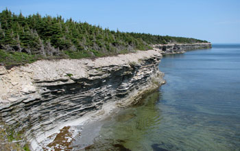
Coastal outcrop exposure of Late Ordovician Ellis Bay Formation, Anticosti Island, Quebec, Canada.
February 17, 2011
In the Late Ordovician Period of Earth's geologic history, about 450 million years ago, more than 75 percent of marine species perished and Earth scientists have been seeking to discover what caused the extinction. It was the second largest in Earth's history.
Now, using a new research method, investigators believe they are closer to finding an answer.
Employing a new way to measure ancient ocean temperatures, a team of researchers at the California Institute of Technology (Caltech) recently discovered a link between ancient climate change and the Late Ordovician mass extinction. The team found the extinction event occurred during a glacial period when global temperatures became cooler and the volume of glacial ice increased.
Both the changes in temperature and the increase of continental ice sheets are factors that could have affected marine life in these ancient waters, said Woodward Fischer, an assistant professor of geobiology at Caltech.
"Our tools are getting better to ask more questions about ancient climate, so we're really shaping our picture of what that world was like," he said.
In the past, measuring ancient ocean temperatures was based on measuring the ratios of oxygen isotopes found in minerals from ocean water. The challenge was knowing the concentration of isotopes in the ocean at that time, which was needed to determine past water temperatures. But, because there is no direct record of the isotopic composition of ancient oceans, it was difficult to determine the water temperature.
The new method, developed in the laboratory of John Eiler, Sharp Professor of Geology and professor of geochemistry at Caltech, determines the temperature of the ocean by examining the spatial organization of isotopes in fossils that existed in the Late Ordovician Period; in particular, the method looks at the extent to which rare isotopes group together into the same chemical unit in a mineral structure.
This new method "requires really well-preserved minerals, so we used fossils," explained Fischer. "Shells are ideal for this technique."
Fossilized marine species shells were used from present-day Quebec, Canada, and from the mid-western United States.
Fischer said the types of species that went extinct during the Late Ordovician Period included mostly benthic invertebrates, or invertebrates that live on the ocean floor and filter plankton for food. These were organisms such as trilobites and brachiopods. Paleozoic corals and cephalopods, which Fisher described as resembling "squids in a tube," were impacted as well. Some vertebrates, primarily fish, also were impacted by the change in global temperature, but fossil evidence of these organisms is less common.
Eiler explained that the findings of this study revealed that during the Late Ordovician, the temperatures of tropical oceans were higher than they are today, but for a brief period, experienced a drop in temperature by five degrees. At the same time, the volume of ice in the poles expanded. After this glacial period, the ocean temperatures rose, and the ice volume returned to its earlier, lower amount.
"We've observed a cycle of climate variability," said Eiler, who explained that these findings can be used to learn more about changes in climate today.
The temperature reconstruction of O’Donnell et al. (2010) confirms that West Antarctica is warming — but underestimates the rate
Eric Steig
At the end of my post last month on the history of Antarctic science I noted that I had an initial, generally favorable opinion of the paper by O’Donnell et al.in the Journal of Climate. O’Donnell et al. is the peer-reviewed outcome of a series of blog posts started two years ago, mostly aimed at criticizing the 2009 paper in Nature, of which I was the lead author. As one would expect of a peer-reviewed paper, those obviously unsupportable claims found in the original blog posts are absent, and in my view O’Donnell et al. is a perfectly acceptable addition to the literature. O’Donnell et al. suggest several improvements to the methodology we used, most of which I agree with in principle. Unfortunately, their actual implementation by O’Donnell et al. leaves something to be desired, and yield a result that is in disagreement with independent evidence for the magnitude of warming, at least in West Antarctica.
In this post, I’ll summarize the key methodological changes suggested by O’Donnell et al., discuss how their results compare with our results, and the implications for our understanding of recent Antarctic climate change. I’ll then try to make sense of how O’Donnell et al. have apparently wound up with an erroneous result.
First off, a reminder for those not familiar with it: the essential innovation in our work was to combine the surface temperature data available from satellites with the ~50 years of data from weather stations. The latter are generally considered more reliable and go back a full 50 years, but are very sparse and incomplete, whereas the satellite data provide complete spatial coverage of the continent, but only since the early 1980s. We combined the two data sets by calibrating the weather station data against the satellite data, and using the calibration to get a complete spatial picture of Antarctic temperature variability and trends for the last 50 years. The key findings were that the overall Antarctic trend was positive (but not necessarily statistically significant), and that in West Antarctica, the trends were both positive and significant, especially in winter and spring. These findings were important enough for Nature to publish them because most researchers thought that significant warming was restricted only to the Antarctic Peninsula region. None of these findings is contradicted by O’Donnell et al.’s results.
O’Donnell et al. have three main criticisms of our work. First, that the reconstruction we reported was not homogenous. That is, the first part of the reconstruction (1957 through 1981) is based entirely on a linear combination of weather station data (since there are no satellite data during that period); while the second part (1982-2006) is derived simply from the satellite data. O’Donnell et al argue that it would be better to use the only weather station data for both periods, since these data are a priori considered more reliable. (There are all sorts of potential problems with the satellite data, the chief one being that there is a ‘clear sky’ bias.) That is, one wants to calibrate the data during 1982-2006, and then use that calibration to model the temperature field for both the early and the later periods, using only the weather stations.
Second, that in doing the analysis, we retain too few (just 3) EOF patterns. These are decompositions of the satellite field into its linearly independent spatial patterns. In general, the problem with retaining too many EOFs in this sort of calculation is that one’s ability to reconstruct high order spatial patterns is limited with a sparse data set, and in general it does not makes sense to retain more than the first few EOFs. O’Donnell et al. show, however, that we could safely have retained at least 5 (and perhaps more) EOFs, and that this is likely to give a more complete picture.
Third, O’Donnell et al. argue that we used too low a truncation parameter when doing the ‘truncated least squares’ regressions. In general, using too low a truncation parameter will overly smooth the results, and tend to smooth both temporal and spatial information. The problem with using too large a truncation parameter is that it creates problems when data are sparse, resulting in numerical noise (overfitting). O’Donnell et al. try to get around this problem by using cross validation — that is, trying a bunch of different truncation parameters, and using the ones that give the maximum r2, RE and CE statistics.
There are a number of other criticisms that O’Donnell et al. make, such as whether it is okay to infill the weather station data at the same time as doing the calibration against the satellite data (as we did) or whether these have to be done separately (as O’Donnell et al. did). These are more technical points that may or may not be generally applicable, but in any case do not make a significant difference to the results at hand (as O’Donnell et al. point out).
Let’s assume, for the moment, that all of these ideas are on the mark, and that the main reconstruction presented by O’Donnell et al. is, in fact, a more accurate picture of Antarctic temperature change in the last 50 years than presented in previous work. What are the implications for Antarctic climate? How would they differ what was concluded in Steig et al. (2009)? The answer is: very little.
The spatial patterns of annual trends, and how they evolve through time, is similar in both papers. In particular, O’Donnell et al. find, as we did, that the entire continent was warming, on average, prior to early 1980s (Figure below from their main “RLS” reconstruction). As we said in our paper, this would tend to support the idea that cooling in East Antarctica is a recent phenomenon at least in part attributable to recent trends in the Southern Annular Mode (SAM), which is itself forced (at least in part) by stratospheric ozone depletion.
O’Donnell et al. also reproduce our finding that the seasons in which the most rapid and significant warming is occurring are winter and spring — in large areas of both East Antarctica and West Antarctica. In spring, warming is significant throughout all of West Antarctica through the entire 50 years of the record, and in winter, it also occurs throughout all of West Antarctica in the last 25 years. In both seasons in this latter period, the locus of greatest warming has been West Antarctica, and particularly the Ross Sea region and Marie Byrd land, not just the Antarctic Peninsula as virtually all studies prior to ours had assumed. This is an important result that we highlighted in our paper because it has implications for our understanding of the dynamics involving Antarctic warming. Specifically, we made a model-data comparison in the paper, in which we said
… both in the reconstruction and in the model results, the rate of warming is greater in continental West Antarctica, particularly in spring and winter, than either on the Peninsula or in East Antarctica…. This is related to SST changes and the location of sea ice anomalies, particularly during the latter period (1979–2003), when they are strongly zonally asymmetric, with significant losses in the WestAntarctic sector but small gains around the rest of the continent.
In other words, during the period where we have good sea ice data, areas with little sea ice are always areas of surface warming in the Antarctic. It was already well established before our work that sea ice anomalies play a major role in the observed waring on the Antarctic Peninsula’s west coast. Our work showed that this is also true in West Antarctica, and is fully confirmed by O’Donnell et al.’s analysis. The only point of disagreement is in winter, in the earlier part of the record only (prior to the satellite era).
Another point of complete agreement between our results and O’Donnell et al. is that the most widespread cooling occurs in fall — not summer as discussed in earlier work (e.g. Thompson and Solomon, 2000). This may be something of a problem for the hypothesis that ozone depletion is a major driver of the observed East Antarctic cooling, because the forcing is occurring in spring (when the ozone hole develops). If there is a link between the spring forcing and fall temperature, it is not a simple one, but likely would include a role for sea ice, which offers an obvious source of persistence from season to season (a paper in review by Arnour and others argues exactly this point).
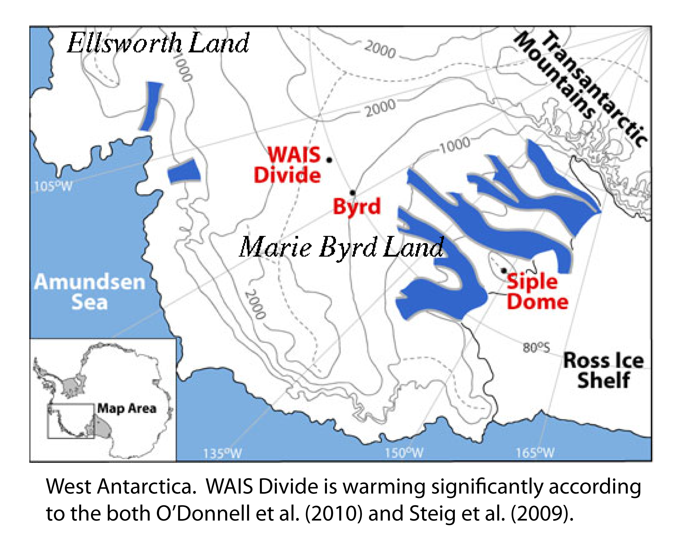
Finally, O’Donnell et al. agree with us on the most basic result of all: there is statistically significant warming in West Antarctica. In this context, it is worth being very clear on what is meant by “West Antarctica”. Reading what has been said about O’Donnell et al. in various places in the blogosphere, one would get the impression that their paper returns the warming of Antarctica to its ‘rightful’ place, the Antarctic Peninsula alone. If that were true, it would certainly be a significant refutation of our work. But in the actual abstract of O’Donnell et al., it is stated that “we find that statistically significant warming extends at least as far as Marie Byrd Land.” Marie Byrd Land is that part of West Antarctica that extends eastward from the Ross Ice Shelf up past Byrd Station and over the central West Antarctic Ice Divide (see the map above). In O’Donnell’s results, there is significant warming all the way from the Peninsula westward past WAIS Divide site, at 112°W, well within Marie Byrd Land and nowhere near the Antarctic Peninsula. Prior to our work, no one had claimed that any area outside the Peninsula was warming significantly. Borehole thermometry at WAIS Divide (Orsi and Severinghaus, 2010) and at the Rutford Ice Stream (closer to the Peninsula; Barrett et al,. 2009) has since provided completely independent validation of these results. O’Donnell et al. is thus merely the latest of several studies to confirm our original finding*: West Antarctica is warming significantly.
To be sure, there is real disagreement between our results and those of O’Donnell et al. For the full fifty year reconstruction of temperature trends, the main reconstruction they discuss in the paper shows cooling in the winter and fall over the Ross Ice Shelf, which contrasts with our finding of significant warming there. As a consequence, their overall warming trends are smaller, by about half. These are the only important differences between our results and those of O’Donnell. Nevertheless, they are significant differences, and certainly may be important for our understanding of Antarctic climate change. In particular both results would tend to suggest a greater role for natural variability than our findings implied. If O’Donnell et al.’s results are correct, this would suggest that the damped response of Antarctica to global radiative forcing (i.e. CO2 increases) that is commonly seen in models (as discussed previously by Spencer Weart, for example) is perhaps more on the mark than our paper would suggest (though note that even the much larger trends we estimated are still significantly damped compared with the Arctic.)
Let’s return now to the question of whether O’Donnell et al.’s results actually do represent an improvement over ours. The figure below indicates a rather glaring problem: O’Donnell et al. disagree markedly with the raw weather station data from Byrd, which is the only record of any length anywhere in West Antarctica. Shown in the figure, reproduced again below, are the main reconstructions of Steig et al. (2009) (green) and O’Donnell et al. (2010) (blue), compared with the the actual raw data (black) from the Byrd weather station. The simple linear trend on the raw data is nearly four times larger in reality than shown by O’Donnell et al., whereas it is not statistically distinguishable from Steig et al. There are a lot of missing data from Byrd (and annual means in the figure include some missing months), so also shown in the figure (dashed) is an independent infilling of missing data from Byrd station, done by Andy Monaghan (using no satellite data whatsoever, as described in Monaghan et al., 2008, plus new data available through 2009). The updated Monaghan estimate — currently under review — indicates an even higher trend, >0.4°C/decade, when the data are updated through 2009.
The evident failure of O’Donnell et al. to correctly capture what is going on at Byrd (and presumably elsewhere in West Antarctica) is quite surprising, given that one of key differences in their methodology is to use the weather station data — not the satellite data as we did — as the verification target. That is, O’Donnell et al. use weather stations, withheld one at a time from the reconstruction for verification purposes to optimize their calibration. How then, can they be so far off for the location of the most important weather station? (I say ‘most important’ here because the main point of contention is, after all, West Antarctica). There are three likely sources of the problem, each pertaining to O’Donnell et al. implementation of their suggested modifications to the method we used.
First, as I noted above, O’Donnell et al. use a linear combination of weather station data for their reconstruction, both in the reconstruction period (pre-1982) and in the calibration period (the satellite era, post 1981). This is a very reasonable thing to do, resulting in a more homogeneous data set than ours. However, it also means throwing out information that might be important: namely, that there are strong trends in the temperatures in West Antarctica that may not be captured by any weather station data. This is not a very large problem in East Antarctica, where the scale of spatial covariance is large, and the number of weather stations is also large; it is a potentially huge problem in West Antarctica, where the number of stations is small (again, only Byrd goes back beyond the satellite era) and the spatial scale of covariance is also smaller, due to the greater topographic relief. On top of that, O’Donnell et al. do not appear to have used all of the information available from the weather stations. Byrd is actually composed of two different records, the occupied Byrd Station, which stops in 1980, and the Byrd AWS station which has episodically recorded temperatures at Byrd since then. O’Donnell et al. treat these as two independent data sets, and because their calculations (like ours) remove the mean of each record, O’Donnell et al. have removed information that might be rather important. namely, that the average temperatures in the AWS record (post 1980) are warmer — by about 1°C — than the pre-1980 manned weather station record. Note that caution is in order in simply splicing these together, because sensor calibration issues could means that the 1°C difference is an overestimate (or an underestimate).** Since Steig et al. retained the satellite data, we didn’t need to worry about this. O’Donnell et al didn’t have that luxury, and should at the very least have considered the impact of treating Byrd Station and Byrd AWS as entirely independent records.
Second, in their main reconstruction, O’Donnell et al. choose to use a routine from Tapio Schneider’s ‘RegEM’ code known as ‘iridge’ (individual ridge regression). This implementation of RegEM has the advantage of having a built-in cross validation function, which is supposed to provide a datapoint-by-datapoint optimization of the truncation parameters used in the least-squares calibrations. Yet at least two independent groups who have tested the performance of RegEM with iridge have found that it is prone to the underestimation of trends, given sparse and noisy data (e.g. Mann et al, 2007a, Mann et al., 2007b, Smerdon and Kaplan, 2007) and this is precisely why more recent work has favored the use of TTLS, rather than iridge, as the regularization method in RegEM in such situations. It is not surprising that O’Donnell et al (2010), by using iridge, do indeed appear to have dramatically underestimated long-term trends—the Byrd comparison leaves no other possible conclusion.
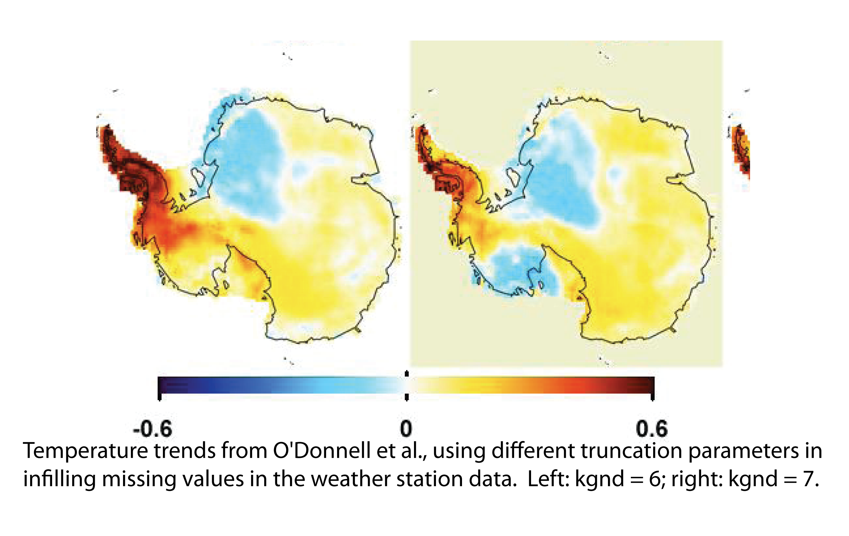
O’Donnell et al. do not rely entirely on ridge regression. They also present results from a more explicit cross-validation test, using various truncation parameters for a ‘truncated total least squares’ (or ‘truncated singular value decompositon’) regressions, as we did in our work. However, these tests, as implemented, are also problematic. O’Donnell et al. actually use cross validation in two steps: first, by filling in missing data in the weather station records and choosing the truncation value (kgnd) that yields the best overall verification statistics. Second, by reconstructing the entire spatial field with another truncation value, ksat. In both cases, the optimization is done on the basis of the entire data set; that is, the ‘best’ parameter depends on what works best on average both in data poor regions (e.g. West Antarctica) and data rich regions (e.g. East Antarctica and the Peninsula). The obvious risk here is that too high a truncation value will be used for West Antarctica. There is rather good evidence to be found in the Supplementary Material in O’Donnell that this is exactly what has happened. The choice of kgnd that yields the best agreement with the iridge calculations (which, remember, is already known to create problems) happens to be kgnd = 7, and it just so happens that this yields the minimum trends. In fact, O’Donnell et al. show in a table in their Supplementary Material that the mean trend for West Antarctica for smaller values of kgnd is more than twice (~0.2 °C/decade) what it is for their ‘optimum’ estimate of kgnd = 7 (~0.07°C/decade). Indeed, using any value lower than the one they choose to rely on largely erases any difference between their results and Steig et al., 2009. This simple fact — illustrated in the figure above (trends in °C/decade for 1957-2006) — has been notably absent in the commentaries that O’Donnell and coauthors have made about their paper.
Third, the way that O’Donnell et al. actually do the cross-validation to optimize ksat is itself pretty dodgy. Rather than using split calibrations (that is, comparing early period with late period statistics), they one-by-one withhold each weather station time series over the entire length of the record. To see the problem with this, consider what happens if you withhold the South Pole station record, which is complete for the entire time period, and then repeat the regressions to find the best truncation value for South Pole. For the period 1982-2006, when there are satellite data available for (and highly correlated with the station at) South Pole, the optimal number will be much higher (data richness) than during the pre-satellite era (data poor). The number that gets used will be an underfitting for the pre-satellite era and an overfitting for the satellite era. Note that ksat is actually the number of EOFs that get retained; since one needs many more of these to reconstruct the Peninsula properly, it is inevitable that they’ll wind up with more retained EOFs than we did; that doesn’t mean this is the right number for West or East Antarctica. O’Donnell et al. do report split calibration statistics as well, but this is not how they choose their optimal values.
Does all of this mean that I think O’Donnell’s results are all wrong? Certainly not. I think that they are right to have retained more EOF patterns than we did, though the main impact of this is only in capturing the strong Peninsula warming.*** It is also quite likely that O’Donnell et al.’s results are more accurate than ours for the satellite era, during which most of the problems I have discussed above are less likely to arise. Although their results show much smaller trends, they agree well with the spatial patterns in weather forecast reanalysis data products (NCEP2, ERA-40) during the satellite era. This is a nice, largely independent validation of those products, and suggests that it is okay to use those products — which include detailed information on atmospheric circulation changes, for example — for investigating the causes of the temperature trends. This is something that quite a few of us have been working on, but there has always been the nagging problem that we don’t really know how much we can trust NCEP and ERA products at high southern latitudes. O’Donnell et al. should certainly be cited in support of such work.
In summary, even if their results are taken at face value, O’Donnell et al. 2010 doesn’t change any of the conclusions reached in Steig et al. In West Antarctica where there is disagreement, Steig et al, 2009 is in better agreement with independent data, and O’Donnell et al.’s results appear to be adversely affected by using procedures known to underestimate trends. Thus while their results may represent an improved estimate for the trends in data rich regions — East Antarctica and the Peninsula — it is virtually certain that they are an underestimate for West Antarctica. This probably means going back to the drawing board to write up another paper, taking into account those suggestions of O’Donnell et al. that are valid, but hopefully avoiding their mistakes.
*Contrary to what Ryan O’Donnell has claimed, Doran et al. (2006) reported warming in Ellsworth Land (between WAIS Divide and the Peninsula) only in winter, with cooling in the annual mean. It is worth noting that Doran’s work has previously been misrepresented, though in the opposite way!
**There is, however, completely independent data from the WAIS Divide borehole, showing that this site has warmed by the same amount indicated by the Byrd weather station data — about 1°C since 1958. This is unpublished data, but the results were presented in an AGU talk and in the published abstract.
*** Peninsula warming was not the question we were addressing in our paper, as we made very clear in the text. We chose fewer EOFs based on our previous work (Schneider et al., 2004) showing that this sufficiently captures both East and West Antarctica.) Although retaining fewer EOFs reduces the spatial details, it is a conservative choice for estimating large-scale trends in both West and East Antarctica. See also our discussion on overfitting.
Friday, February 4, 2011
Extinctions breed carbon chaos
Massive die-offs left ecosystems vulnerable, analysis suggests
Big extinctions don’t just wipe out a lot of species. They also send ecological cycles reeling for millions of years, a new study suggests.
Following massive die-offs, the natural processes that keep carbon flowing through marine ecosystems — from tiny photosynthesizers to big fish and between the bottom and the top of the ocean — get broken. For millions of years after at least two global disasters, marine communities were too unstable to keep the molecules churning, researchers report in the February issue of Geology. These “chaotic carbon episodes” could have big ramifications for extinctions in the modern era, say scientists from Brown University in Providence, R.I., and the University of Washington in Seattle.
In healthy marine ecosystems, diverse swimming predators, lazy filter feeders and myriad other organisms keep the carbon flowing nonstop, says study coauthor Jessica Whiteside, a paleobiologist at Brown. But after a global extinction, when only a few plants, animals or single-celled critters occupy each rung of the food chain, minicatastrophes like diseases or climatic shifts take big tolls, she says. “If you already have a weakened state of ecosystems, these things that would normally be minor variations now become wildly oscillating,” she says.
The team looked particularly at the diversity of ancient octopus-like animals called ammonites, which were ultimately wiped out by the same extinction that killed the dinosaurs. Ammonites often swam to catch prey as well as floated idly, snagging debris from ocean currents. But for millions of years after the end-Permian mass extinction 250 million years ago, as well as after the end-Triassic mass extinction 50 million years later, few swimming ammonites survived.
The devastation of ammonites and other life forms left its mark on the geologic record, Whiteside says. Scientists recognize five mass extinctions in Earth’s history. The worst — the end-Permian extinction — killed about 90 percent of ocean-dwelling species. Scientists discovered that after most of these calamities carbon molecules in the environment, on average, got lighter. The culprits behind this drop are major volcanic events like those associated with the end-Permian mass extinction. Volcanoes spew a relatively high proportion of lighter isotopes of carbon — atoms with fewer neutrons in their nuclei — into the atmosphere, says Jean Guex, a paleobiologist with Lausanne University in Switzerland.
“They are not volcanoes like people imagine,” says Guex, who was not involved in either study. “They are fissures which are extruding millions of cubic kilometers of basalts, inducing major atmospheric pollutions with sulfur and heavy metals.”
Tiny photosynthesizers gobble down the lighter carbon in the air, introducing it to the environment and, eventually, the geologic record. In a normally functioning ecosystem, that would cause the proportion of light carbon isotopes in the record to lighten and then eventually return to normal. But when Whiteside’s team eyed carbon isotopes in sedimentary layers from the periods following the end-Permian extinction and the end-Triassic extinction, carbon weights jumped back and forth from heavier to lighter isotopes. She argues that ecosystem instabilities could easily have triggered these wild fluxes. As living organisms died, they floated to the ocean bottom, carrying the lighter carbon molecules in their bodies with them. That left the carbon in the surface waters, on average, heavier, she says. When communities rebounded, carbon weights in the upper oceans dropped back down.
But Guex says that the real chaotic factor in this picture was the environment, not the carbon flows. Undersea volcanoes erupted on and off for millions of years following each extinction event, he argues. “The carbon isotopes mainly reflect these crises.”
Whiteside agrees that such churning could have played a role but cautions against ignoring the ecological factors. Minor volcanic eruptions would have affected weak communities much more than strong ones, she says.
The team’s conclusions are particularly relevant for the modern era — what many biologists have dubbed the sixth mass extinction, Whiteside notes. Computer simulations of climate change look 100 years into the future, but the impacts of species extinctions today may last long after human pollution has come and gone, she says. “It’s a cautionary tale for the species loss that’s going on right now.”


 In this post, I’ll summarize the key methodological changes suggested by O’Donnell et al., discuss how their results compare with our results, and the implications for our understanding of recent Antarctic climate change. I’ll then try to make sense of how O’Donnell et al. have apparently wound up with an erroneous result.
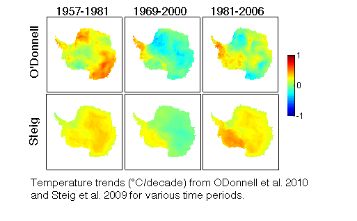

 Another point of complete agreement between our results and O’Donnell et al. is that the most widespread cooling occurs in fall — not summer as discussed in earlier work (e.g.
 O’Donnell et al. do not rely entirely on ridge regression. They also present results from a more explicit cross-validation test, using various truncation parameters for a ‘truncated total least squares’ (or ‘truncated singular value decompositon’) regressions, as we did in our work. However, these tests, as implemented, are also problematic. O’Donnell et al. actually use cross validation in two steps: first, by filling in missing data in the weather station records and choosing the truncation value (kgnd) that yields the best overall verification statistics. Second, by reconstructing the entire spatial field with another truncation value, ksat. In both cases, the optimization is done on the basis of the entire data set; that is, the ‘best’ parameter depends on what works best on average both in data poor regions (e.g. West Antarctica) and data rich regions (e.g. East Antarctica and the Peninsula). The obvious risk here is that too high a truncation value will be used for West Antarctica. There is rather good evidence to be found in the Supplementary Material in O’Donnell that this is exactly what has happened. The choice of kgnd that yields the best agreement with the iridge calculations (which, remember, is already known to create problems) happens to be kgnd = 7, and it just so happens that this yields the minimum trends. In fact, O’Donnell et al. show in a table in their Supplementary Material that the mean trend for West Antarctica for smaller values of kgnd is more than twice (~0.2 °C/decade) what it is for their ‘optimum’ estimate of kgnd = 7 (~0.07°C/decade). Indeed, using any value lower than the one they choose to rely on largely erases any difference between their results and Steig et al., 2009. This simple fact — illustrated in the figure above (trends in °C/decade for 1957-2006) — has been notably absent in the commentaries that O’Donnell and coauthors have made about their paper.